Question
Obtain the equations of motion of coupled pendulum (two pendulums connected by a spring) using the Lagrangian method.
Solution
Consider a system of coupled pendulums as shown below in the figure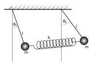
The displacement of A is $x_{1}$ and B is $x_{2}$ , condition being \({x_1}\) < \({x_2}\).
In such state the spring gets stretched. The lengths of the strings of both the pendulums are same (say l).
The angular displacement of A is \({\theta _1}\) and that of B is \({\theta _2}({\theta _2} > {\theta _1})\).
Therefore
\(\begin{array}{l}{x_1} = l{\theta _1} \Rightarrow {\theta _1} = \frac{{{x_1}}}{l}{\rm{ (1)}}\\{x_2} = l{\theta _2} \Rightarrow {\theta _2} = \frac{{{x_2}}}{l}{\rm{ (2)}}\end{array}\)
As the spring gets stretched, it is clear from the figure that restoring force works along the direction of displacement\({\theta _1}\) and opposite to the direction of displacement \({\theta _2}\) .
Now A and B at zero potential level, the total potential energy of the system is given as
\(V = mgl(1 – \cos {\theta _1}) + mgl(1 – \cos {\theta _2}) + \frac{1}{2}k{({x_2} – {x_1})^2}\)
Where m is the mass of each one of the bob and k is the spring constant.
Since \({\theta _1}\)and \({\theta _2}\)are small so,
\(\begin{array}{l}\cos {\theta _1} = 1 – \frac{{\theta _1^2}}{2} + \frac{{\theta _1^4}}{4} + ……\\\cos {\theta _2} = 1 – \frac{{\theta _2^2}}{2} + \frac{{\theta _2^4}}{4} + ……\end{array}\)
Neglecting the higher powers other than squares of \({\theta _1}\)and \({\theta _2}\)the expression of potential energy can be written as
\(\begin{array}{l}V = mgl\frac{{\theta _1^2}}{2} + mgl\frac{{\theta _2^2}}{2} + \frac{1}{2}k{({x_2} – {x_1})^2}\\{\rm{ = }}\frac{{mgx_1^2}}{{2l}} + \frac{{mgx_2^2}}{{2l}} + \frac{1}{2}k{({x_2} – {x_1})^2}\end{array}\)
Also the kinetic energy of whole system is
\(T = \frac{1}{2}m\dot x_1^2 + \frac{1}{2}m\dot x_2^2 = \frac{1}{2}m(\dot x_1^2 + \dot x_2^2)\)
Hence Lagrangian L would be
\(\begin{array}{l}L = T – V \\L = \frac{1}{2}m(\dot x_1^2 + \dot x_2^2) – \frac{{mgx_1^2}}{{2l}} – \frac{{mgx_2^2}}{{2l}} – \frac{1}{2}k{({x_2} – {x_1})^2}\end{array}\)
Now
\(\begin{array}{l} \frac{\partial L}{\partial {{x}_{1}}}=-\frac{mg{{x}_{1}}}{l}+k({{x}_{2}}-{{x}_{1}}) \\\end{array}\)
\(\begin{array}{l}\frac{\partial L}{\partial {{{\dot{x}}}_{1}}}=m{{{\dot{x}}}_{1}} \\\end{array}\)
\(\begin{array}{l}\therefore \frac{d}{dt}\left( \frac{\partial L}{\partial {{{\dot{x}}}_{1}}} \right)=\frac{d}{dt}(m{{{\dot{x}}}_{1}})=m{{{\ddot{x}}}_{1}} \\\end{array}\)
Hence Lagrangian equation in terms of \({x_1}\)is
\(\begin{array}{l}\frac{d}{{dt}}\left( {\frac{{\partial L}}{{\partial {{\dot x}_1}}}} \right) – \frac{{\partial L}}{{\partial {x_1}}} = 0\\or,\\m{{\ddot x}_1} + \frac{{mg{x_1}}}{l} – k({x_2} – {x_1}) = 0\\or,\\m{{\ddot x}_1} = – \frac{{mg{x_1}}}{l} + k({x_2} – {x_1})\end{array}\)
Also,
\(\begin{array}{l}\frac{{\partial L}}{{\partial {x_2}}} = – \frac{{mg{x_2}}}{l} – k({x_2} – {x_1})\\\frac{{\partial L}}{{\partial {{\dot x}_2}}} = m{{\dot x}_2}\\and\\\frac{d}{{dt}}\left( {\frac{{\partial L}}{{\partial {{\dot x}_2}}}} \right) = m{{\ddot x}_2}\end{array}\)
Hence Lagrangian equation in terms of \({x_2}\)is
\(\begin{array}{l}\frac{d}{{dt}}\left( {\frac{{\partial L}}{{\partial {{\dot x}_2}}}} \right) – \frac{{\partial L}}{{\partial {x_2}}} = 0\\or,\\m{{\ddot x}_2} = – \frac{{mg{x_2}}}{l} – k({x_2} – {x_1})\end{array}\)
The equation of motion for given system are
\(\begin{array}{l}m{{\ddot x}_1} = – \frac{{mg{x_1}}}{l} + k({x_2} – {x_1})\\m{{\ddot x}_2} = – \frac{{mg{x_2}}}{l} – k({x_2} – {x_1})\end{array}\)