A picture is worth a thousand numbers. The position-time graph turns a data table into a visual story — you can read velocity, rest, and acceleration just from the shape of the line. From NCERT Chapter 4 (Exploration edition) Class 9 Science. Aligned with CBSE syllabus 2026-27.

Q. Why do we draw graphs to study motion?
A table of (time, position) values tells you what happened, but it is hard to see the pattern at a glance. A position-time graph converts that data into a visual picture — the shape of the line immediately reveals whether the object is at rest, moving uniformly, or accelerating. You can extract velocity from the slope and compare multiple objects on the same axes.
A position-time graph (also called a distance-time graph when motion is in one direction) is a graph in which:
Each point $(t, s)$ on the graph tells you: "At time $t$, the object was at position $s$." Joining the points gives a line or curve — its shape encodes the entire story of the motion.
Q. What is the origin in a position-time graph?
The origin O is the point (0, 0) — the starting position at time zero. Not every object starts at the origin; a graph can start at a non-zero position if the object was already away from the reference point at the beginning of observation.
NCERT Activity 4.3 asks you to plot a position-time graph for a uniformly moving vehicle using recorded data. Here is the step-by-step method.
| Time (s) | Position (m) |
|---|---|
| 0 | 0 |
| 2 | 40 |
| 4 | 80 |
| 6 | 120 |
| 8 | 160 |
Step 1 — Draw the axes: Draw two perpendicular lines. The horizontal line is the x-axis (time); the vertical line is the y-axis (position). Mark the point where they meet as the origin O (0, 0).
Step 2 — Choose a scale: The scale must fit all data on the graph paper without crowding. A common NCERT choice: x-axis: 5 small divisions = 1 s (so 10 divisions = 2 s, etc.); y-axis: 5 small divisions = 20 m (so 2 divisions = 8 m, etc.). Write the scale at the top corner.
Step 3 — Label the axes: Write "Time (s)" along the x-axis and "Position (m)" along the y-axis with arrows indicating the positive direction.
Step 4 — Plot the data points: For each row in the table, locate the time on the x-axis and the corresponding position on the y-axis, then mark the point with a small cross (×) or dot. Points to plot: (0, 0), (2, 40), (4, 80), (6, 120), (8, 160).
Step 5 — Join the points: If the points lie on a straight line, use a ruler and draw a single straight line through all of them. If the points follow a curve, draw a smooth curve (do not connect point-to-point with zigzag lines).
For the Table 4.3 data, the points lie perfectly on a straight line passing through the origin — confirming that the vehicle is in uniform motion.
Q. How do we read the type of motion from the graph?
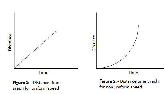
The shape of the line or curve on a position-time graph is a direct fingerprint of the type of motion.
When equal distances are covered in equal time intervals, the position increases linearly with time. The graph is a straight line passing through the origin. The steeper the line, the higher the velocity.
Example: Table 4.3 data above — vehicle covering 40 m every 2 s gives a straight line. Velocity = constant = slope of the line.
When velocity is increasing (accelerated motion), the object covers more and more distance in each successive time interval. The points no longer lie on a straight line — they bend upward. The graph is a concave-upward curve.
Example: NCERT Example 4.5 — accelerating vehicle from Table 4.4 — the position increases faster and faster, giving an upward-curving graph.
If the position does not change with time, the graph is a horizontal line (parallel to the x-axis). The object is stationary — its velocity is zero (slope = 0).
Example: NCERT Example 4.6 — a vehicle parked at 40 m from the reference point. Its position remains 40 m for all values of $t$. Slope = 0, velocity = 0.
When two objects are both in uniform motion, the one with the steeper slope has the higher velocity — it covers more distance per unit time.
Example: NCERT Example 4.7 — objects A and B, both moving uniformly, plotted on the same axes. Object B has a steeper slope → higher velocity than A.
| Graph Shape | Type of Motion | Velocity |
|---|---|---|
| Straight line through origin (gentle slope) | Uniform motion | Low, constant |
| Straight line through origin (steep slope) | Uniform motion | High, constant |
| Horizontal line (any height) | At rest | Zero |
| Curve bending upward (concave up) | Accelerated (non-uniform) motion | Increasing |
| Curve bending downward (concave down) | Decelerated (non-uniform) motion | Decreasing |
Q. How do we calculate velocity from a position-time graph?
The slope of any straight-line graph is defined as (change in y) ÷ (change in x). For a position-time graph:
Where on the graph, $BC$ is the vertical side (change in position) and $CA$ is the horizontal side (change in time) of the right-angled triangle formed by choosing two points on the line.
Using the Table 4.3 data: choose the points $(t_1 = 2 \text{ s},\, s_1 = 40 \text{ m})$ and $(t_2 = 4 \text{ s},\, s_2 = 80 \text{ m})$:
$$v = \frac{s_2 - s_1}{t_2 - t_1} = \frac{80 - 40}{4 - 2} = \frac{40}{2} = 20 \text{ m s}^{-1}$$You can use any two points on the line and get the same slope — because uniform motion has constant velocity. Try $(0, 0)$ and $(8, 160)$: slope = 160/8 = 20 m s⁻¹. Same answer.
For a curved position-time graph (accelerated motion), the slope changes at every point — it equals the instantaneous velocity at that point. To find the slope at a point on a curve, draw a tangent to the curve at that point and calculate the slope of that tangent. This is a graphical method you will practise in Activity 4.4.
Velocity is defined as displacement ÷ time. On a position-time graph, the y-axis is position (displacement from the reference) and the x-axis is time. So any ratio of (vertical change) ÷ (horizontal change) is literally displacement ÷ time = velocity. The slope is the graphical representation of the formula — this is why graphs are so powerful. They turn an equation into a visible geometric property.
A vehicle starts from rest and records the following positions:
| Time (s) | 0 | 2 | 4 | 6 | 8 |
|---|---|---|---|---|---|
| Position (m) | 0 | 10 | 40 | 90 | 160 |
Observation: The position does not increase by the same amount in each 2-second interval (10, 30, 50, 70 m — increasing increments). The vehicle covers more distance each second — it is accelerating. When plotted, the points form an upward-curving parabola, not a straight line.
Why the curve bends upward: The slope at each successive point is greater than the previous one, because velocity is increasing. A steeper slope at later times means higher velocity at those times — which is the visual signature of acceleration.
A vehicle is parked at a position of 40 m from the reference point. Regardless of how much time passes, its position remains 40 m. The graph is a horizontal line at $s = 40$ m.
Slope = 0, therefore velocity = 0. The horizontal line is the graphical representation of "no motion."
Yes — if the object moves in the negative direction (back past the origin), its position becomes negative. A position-time graph can dip below the x-axis for an object that returns behind its starting reference point.
Two objects A and B are both in uniform motion, plotted on the same position-time graph. Object B has a steeper line than Object A.
Question: Which has higher velocity?
Object B has the higher velocity because its line is steeper — it has a larger slope. In the same time interval, B covers more distance than A. You can confirm this by calculating the slope of each line using two points and comparing the numbers.
Students often think of a position-time graph as a picture of the road or path the object travelled — like a map viewed from above. This is incorrect.
A position-time graph shows how position changes with time — it is a mathematical graph, not a physical drawing of the route. The y-axis is position (a number), not a direction in space.
Example: If an object moves along a straight east-west road and reverses direction, the position-time graph may look like a hill (position increases then decreases). The graph looks curved, but the road is perfectly straight. The graph tells you where the object was at each moment, not what path it drew on a map.
These two terms are often used interchangeably in Class 9, and in many practical cases they represent the same graph. Here is when they are the same and when they differ:
| Aspect | Position-Time Graph | Distance-Time Graph |
|---|---|---|
| Y-axis quantity | Position (can be negative) | Distance (always positive) |
| Can graph go below x-axis? | Yes (if object moves past origin) | No (distance never negative) |
| Same when motion is… | One direction only, no reversal — in this case position = distance, so both graphs are identical | |
| Slope gives | Velocity (can be negative) | Speed (always positive) |
For NCERT Class 9 problems (straight-line motion in one direction), both graphs are identical and the terms are used interchangeably.
| What you want to know | How to read it from the graph |
|---|---|
| Position at any instant | Read y-value at that time ✓ |
| Velocity (uniform motion) | Calculate slope = (Δs)/(Δt) ✓ |
| Whether motion is uniform | Straight line → uniform ✓ |
| Whether motion is accelerated | Curve (concave up) → accelerated ✓ |
| Whether object is at rest | Horizontal line (slope = 0) → at rest ✓ |
| Which object is faster | Steeper slope → higher velocity ✓ |
Q1. A position-time graph is a straight horizontal line at $s = 25$ m. What can you conclude about the object's motion?
The object is stationary (at rest) at a position 25 m from the reference point. Its velocity is zero because the slope of a horizontal line is zero. This is NCERT Example 4.6 type situation.
Q2. Two objects P and Q are plotted on the same position-time graph. P's line has a slope of 15 m s⁻¹ and Q's line has a slope of 25 m s⁻¹. Which is faster? How much faster?
Q is faster (steeper slope = higher velocity). Q is faster by 25 − 15 = 10 m s⁻¹.
Q3. A position-time graph shows a straight line, then a horizontal segment, then another straight line. Describe the complete motion.
Phase 1 (straight line): the object moves at constant velocity (uniform motion). Phase 2 (horizontal segment): the object is stationary — it has stopped. Phase 3 (another straight line): the object resumes uniform motion. The velocity in Phase 3 could be the same, higher, lower, or in the opposite direction depending on the slope.
Q4. A vehicle has the following position-time data: at $t = 0$ s, $s = 0$ m; at $t = 5$ s, $s = 100$ m; at $t = 10$ s, $s = 200$ m. Plot points and calculate the velocity.
The three points lie on a straight line (uniform motion). Velocity = slope:
$$v = \frac{100 - 0}{5 - 0} = \frac{100}{5} = \mathbf{20 \text{ m s}^{-1}}$$Verify: (200 − 0)/(10 − 0) = 20 m s⁻¹. Same answer from any two points — confirming uniform motion.
P1. Plot a position-time graph for an object that is at rest at $s = 30$ m from $t = 0$ to $t = 5$ s. What does the graph look like?
A horizontal straight line at $s = 30$ m, from $t = 0$ to $t = 5$ s. The slope is zero (velocity = 0).
P2. Plot the position-time graph for a vehicle with: $t$ (s) = 0, 1, 2, 3, 4; $s$ (m) = 0, 5, 20, 45, 80. Is this uniform or non-uniform motion? Explain using the differences between successive positions.
Successive position differences: 5, 15, 25, 35 — increasing, not constant. This is non-uniform (accelerated) motion. When plotted, the points form an upward-curving parabola (not a straight line).
P3. On the same axes, sketch position-time graphs for two vehicles: Vehicle X with speed 10 m/s and Vehicle Y with speed 20 m/s, both starting from the origin. Which line is steeper? When has Y doubled the distance of X?
Y has a steeper line (higher velocity = steeper slope). Since Y always moves at twice the speed of X, Y is always at double the position of X at any given time $t$. There is no single moment when Y "doubles" X's distance — Y's position is always $2 \times$ X's position throughout the journey.