Introduction
In physics, equilibrium refers to a balanced state where the net force and net torque acting on a body are zero. This concept helps us understand why objects either remain at rest or move with constant velocity.
When studying mechanics, we encounter two primary types of equilibrium based on the motion characteristics of objects.
- Static Equilibrium
- Dynamic Equilibrium
What is Static Equilibrium?
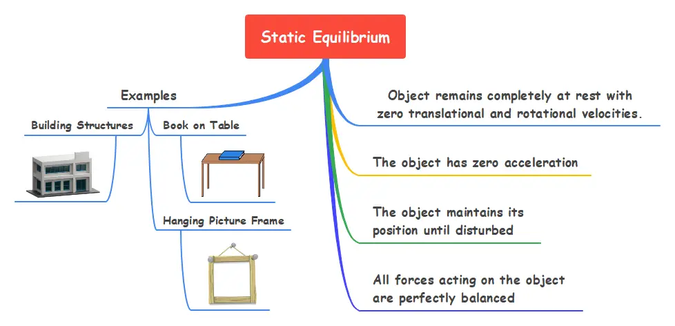
Static equilibrium occurs when an object remains completely at rest with zero translational and rotational velocities. In this state, the object experiences no acceleration in any direction, maintaining its position indefinitely unless disturbed by external forces.
Key Characteristics
In this state:
- The object has zero velocity
- The object has zero acceleration
- All forces acting on the object are perfectly balanced
- The object maintains its position until disturbed
Mathematical Conditions for Static Equilibrium
For an object to be in static equilibrium, two fundamental conditions must be satisfied:
First Condition (Translational Equilibrium):
$\sum F_x = 0, \quad \sum F_y = 0, \quad \sum F_z = 0$
This means the sum of forces in each direction equals zero.
Second Condition (Rotational Equilibrium):
$\sum \tau = 0$
The sum of all torques about any point must be zero.
Examples of Static Equilibrium
Consider these everyday examples of static equilibrium:
- Book on Table: A book resting on a horizontal surface experiences two forces – its weight (mg) downward and normal force (N) upward. Since N = mg, the net force is zero.
- Hanging Picture Frame: The tension in the string balances the picture’s weight, keeping it motionless on the wall.
- Building Structures: Bridges and buildings represent complex static equilibrium systems where all structural forces balance perfectly.
Understanding Dynamic Equilibrium
Dynamic equilibrium describes objects moving at constant velocity while experiencing zero acceleration. This state occurs when forces acting on a moving object perfectly balance, allowing continued motion without speed or direction changes.
Newton’s First Law of Motion directly relates to dynamic equilibrium: an object in motion continues moving uniformly unless acted upon by unbalanced forces. The mathematical conditions remain identical to static equilibrium, but the object possesses constant velocity rather than remaining at rest.
Key Characteristics
- Object moves with constant velocity
- Net force acting on the object equals zero
- No acceleration occurs
- Forces are balanced despite the motion
Mathematical Framework
The mathematical conditions for dynamic equilibrium remain identical to static equilibrium:
$\sum \vec{F} = 0 \quad \text{and} \quad \sum \vec{\tau} = 0$
However, the object possesses constant velocity rather than remaining at rest.
Real-World Examples of Dynamic Equilibrium
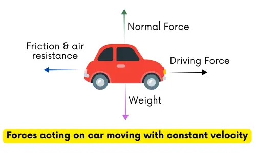
Car at Constant Speed: When driving on a straight highway at steady 80 km/h, the engine force balances air resistance and friction, resulting in zero net force.
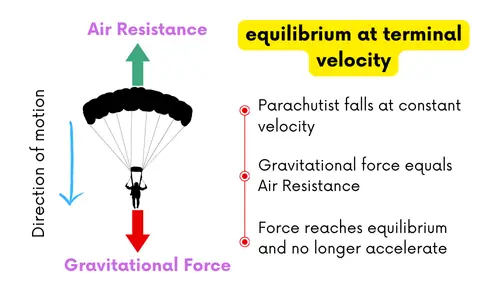
Terminal Velocity: A falling parachutist reaches dynamic equilibrium when gravitational force equals air resistance, causing constant downward velocity.
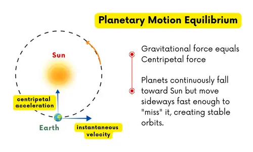
Planetary Motion: Earth maintains dynamic equilibrium in its orbit around the Sun, where gravitational attraction provides exactly the centripetal force needed for uniform circular motion.
Problem-Solving Approach for Equilibrium
Step-by-Step Method
Step 1: Create Free Body Diagram
- Isolate the object under analysis
- Identify all external forces acting on the object
- Draw force vectors with proper directions and magnitudes
Step 2: Choose Coordinate System
- Select convenient x and y axes
- Resolve forces into components when necessary
Step 3: Apply First Condition
- Set sum of forces in x-direction equal to zero
- Set sum of forces in y-direction equal to zero
- Solve the resulting equations
Step 4: Apply Second Condition (if needed)
- Choose a convenient point for torque calculations
- Set sum of torques equal to zero
- Solve for unknown quantities
Key Points to Remember
- Equilibrium ? Rest: Objects can be in equilibrium while moving at constant velocity
- Reference Frame Matters: Equilibrium depends on the chosen reference frame
- Both Conditions Required: For complete equilibrium, both force and torque conditions must be satisfied
- Vector Nature: Forces and torques are vectors and must be treated accordingly
Conceptual Insights for Enhanced Understanding
Equilibrium vs. Rest: A common misconception equates equilibrium with rest. However, dynamic equilibrium demonstrates that motion and equilibrium coexist when forces balance perfectly.
Reference Frame Dependency: Equilibrium depends on the chosen reference frame. An object in dynamic equilibrium relative to Earth might not be in equilibrium relative to an accelerating vehicle.
Pseudo-Forces: In non-inertial reference frames, pseudo-forces (fictitious forces) must be included in equilibrium analysis to account for the frame’s acceleration.
Static vs Dynamic Equilibrium – Comparison Table
| Aspect | Static Equilibrium | Dynamic Equilibrium |
|---|---|---|
| Definition | Object remains completely at rest with zero velocity and acceleration | Object moves with constant velocity while experiencing zero acceleration |
| Motion State | No movement – object is stationary | Uniform motion at constant velocity |
| Velocity | $ v = 0 $ | $ v = \text{constant} \neq 0 $ |
| Acceleration | $ a = 0 $ | $ a = 0 $ |
| Force Condition | Net force $ = 0 $ ($ \sum \vec{F} = 0 $) | Net force $ = 0 $ ($ \sum \vec{F} = 0 $) |
| Torque Condition | Net torque $ = 0 $ ($ \sum \vec{\tau} = 0 $) | Net torque $ = 0 $ ($ \sum \vec{\tau} = 0 $) |
| Component Analysis | $ \sum F_x = 0$, $\sum F_y = 0$, $\sum F_z = 0 $ | $ \sum F_x = 0$, $\sum F_y = 0$, $\sum F_z = 0 $ |
| Time Dependency | Remains constant over time until disturbed | Maintains constant velocity over time |
| Energy State | Energy is conserved with no energy conversion | Continuous energy flow through the system |
| Mathematical Representation | $ v = 0, a = 0$, $\sum \vec{F} = 0$, $\sum \vec{\tau} = 0 $ | $ v = \text{constant}$, $a = 0, \sum \vec{F} = 0$, $\sum \vec{\tau} = 0 $ |
| Examples | – Book resting on table – Person standing still – Building structures – Hanging chandelier | – Car at constant speed – Terminal velocity of falling object – Earth’s orbital motion – Object sliding with constant velocity |
| Response to Disturbance | Any external force disrupts equilibrium and causes motion | External forces are already balanced during motion |
| Newton’s First Law | Object at rest remains at rest | Object in motion continues in uniform motion |
| System Requirements | Can occur in open or closed systems | Typically occurs in systems with balanced opposing forces |
| Stability | Stable until external force is applied | Stable as long as forces remain balanced |
| Application Areas | Structural engineering, architecture, statics problems | Vehicle dynamics, fluid flow, orbital mechanics |
Conclusion
Static and dynamic equilibrium distinguishes between balanced forces in stationary and uniformly moving systems.
The mathematical conditions $\sum \vec{F} = 0$ and $\sum \vec{\tau} = 0$ serve as powerful analytical tools for examining everything from simple objects to sophisticated structures.